Error and Uncertainty
If your experiment needs statistics, you ought to have done a better experiment.
—Ernest Rutherford
The following book in highly recommended and gives a good treatment of error analysis and the propagation of uncertainties: An Introduction to Error Analysis, J.R. Taylor, University Science Books (1996) .
Why consider uncertainty?
An estimate of uncertainty given us an idea of how much confidence you can have in the value of a quantity.
Scenario 1:
Your are trying to budget for the upcoming year and have asked your junior engineers to examine process pricing for you.
Which information would you rather have?
The cost will be $256,000.
The cost will be $256,000 with an uncertainty of $150,000.
Scenario 2:
You are the project manager for development of a new drug.
Your technicians tell you that drug 1 has an efficacy of \(2.5\) and drug 2 has an efficacy of \(3.2\). They tell you that drug 2 is clearly superior and to move ahead with the trials. Upon examination of the data, you find that the uncertainty in the efficacy numbers is \(0.7\). What do you do?
Scenario 3:
Your physician recommends increasing your intake of fruits and vegetables from two servings a day to six to reduce your risk of coronary heart disease and hands you a glossy pamphlet containing the following plot.
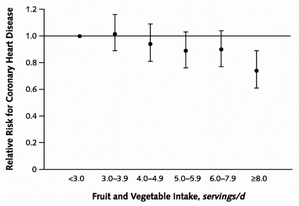
How will this visit change your behavior?
Here are some materials related to error and uncertainty analyses:
Proper specification of a quantity
Three elements must be present:
‘best estimate’ of the value,
uncertainty in the value, and
appropriate units
The standard form for reporting a measurement of a physical quantity \(x\) is
For example, \(\SI{3.49 +- 0.02}{m/s}\).
Thus,
where \(x_{best}\) is the ‘best estimate for \(x\)’ and \(\delta x\) is the ‘uncertainty or error in the measurement’
This statement expresses our confidence that the correct value of \(x\) probably lies in (or close to) the range from \(x_{best} - \delta x\) to \(x_{best} - \delta x\).
If \(x\) is measured in the standard form \(x_{best} \pm \delta x\), the fractional uncertainty in \(x\) is as follows:
Estimating uncertainties
For estimating uncertainty when reading scales and using values from textbooks, papers, and handbooks,
see the procedures in this document.
For estimating uncertainty for repeated measures,
see the procedures in this document.
Stating uncertainties
There are two important rules to when presenting quantities with uncertainties:
Experimental uncertainties should almost always be rounded to one significant figure.
The last significant figure in any stated answer should usually be of the same order of magnitude (in the same decimal position) as the uncertainty.
Examples of applying the rules
incorrect |
correct |
|---|---|
\(\SI{9.82 +- 0.02385}{m/s^{2}}\) |
\(\SI{9.82 +- 0.02}{m/s^{2}}\) |
\(\SI{6051.78 +- 30}{m/s}\) |
\(\SI{6050 +- 30}{m/s}\) |
If our measured quantity is \(\SI{92.81}{cm/s}\), but the uncertainty differs:
uncertainty |
proper representation |
|---|---|
\(\SI{0.32}{cm/s}\) |
\(\SI{92.8 +- 0.3}{cm/s}\) |
\(\SI{3.6}{cm/s}\) |
\(\SI{93 +- 4}{cm/s}\) |
\(\SI{31.9}{cm/s}\) |
\(\SI{90 +- 30}{cm/s}\) |
Propagation of uncertainties
When you combine (add, subtract, multiple, divide) measurements with uncertainties, the uncertainties propagate. The uncertainty of the combined or calculated quantity will always be larger than that of any of the individual uncertainties.
The following rules apply for propagating uncertainties where the individual uncertainties are independent.
Rule for the adding or subtracting quantities with uncertainties
Example
Compute \((3.2 \pm 0.1) – (5.21 \pm 0.03) – (17.2 \pm 0.8)\)
Therefore, the answer, using appropriate significant figures, is
Rule for the multiplying or dividing quantities with uncertainties
Example
Compute \((3.2 \pm 0.1) \times (5.21 \pm 0.03) / (17.2 \pm 0.8)\)
Therefore, the answer, using appropriate significant figures, is
Rule for taking quantities with uncertainties to a power
\[q = x^{n}\]\[\frac{\delta q}{|q|} = |n| \frac{\delta x}{|x|}\]
Example
Compute \(1/\sqrt{7.1 \pm 0.3}\)
The answer, using appropriate significant figures, is then
Other rules
Other rules for exponents, special functions, etc. of numbers with uncertainties are contained in most books on uncertainty analysis, including An Introduction to Error Analysis, J.R. Taylor, University Science Books (1996).
Software
Once you understand the principle of error propagation and how to conduct an error propagation by hand, software can be used to make this task easier, especially for very long series of calculations.
Some relevant software applications are listed in the Wikipedia. page. Unfortunately, many of the links are currently dead.
Other packages for error propagation are available for use in python and MATLAB
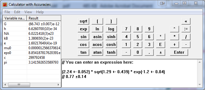
On the Windows OS, a simple to use application is Abacus: a Calculator with Accuracies .
A more flexible (albeit more complex to use) choice on the Windows OS is the GUM Tree Calculator (GTC) .
Exercise
You plan to add a chemical to a large pool and wish to estimate the resulting concentration. You have a scale, a crude tape measure, and a bucket containing the chemical.
The pool is rectangular in cross section and has a constant depth.
The pool is initially empty, but will eventually be completely filled with water.
How will you estimate the concentration?
The relevant concentration units are \(\si{g_{chemical}/l_{water}}\) (\(\SI{1}{m^3}= \SI{1000}{l}\))
You measure the dimensions of the pool and find the following:
You made the following measurements for the chemical mass:
mass of the bucket with the chemical: \(\SI{35.3 +- 0.1}{kg}\)
mass of the empty bucket: \(\SI{4.8 +- 0.2}{kg}\)
What is the concentration of chemical in the pool ( \(\si{g_{chemical}/l_{water}}\) ) and what is the percent uncertainty in this measurement?