Mechanical Energy Balances¶

The scientist describes what is; the engineer creates what never was.

—Theodore von Kármán

Theodore von Kármán had many famous mathematical ancestors and a few notable mathematical descendants. ☺

We had previously considered both heat and work when we formulated our generalized form of the conservation of energy equation.

The Bernoulli equation¶

Utilizing this general equation, we now make the following assumptions:

we have a single input and a single output stream
rate of work and heat effects are negligible compared to other energy-related terms
changes in density are insignificant (incompressible flow)
the velocity adjustment factor, \(\alpha\), is unity
the internal energy consists of ‘rate of flow’ work only

Under these conditions, we arrive at the Bernoulli Equation, which is often employed in engineering to relate velocities and pressures in various types of flows.

Bernoulli equation

Letting \(v_{avg}^{2} = v^{2}\),

\[\left(\frac{P}{\rho} + \frac {1}{2} \, v^{2} + g \, z \right)_{2} - \left(\frac{P}{\rho} + \frac {1}{2} \, v^{2} + g \, z \right)_{1} = 0\]

\[\frac{P_{2} - P_{1}}{\rho} + \frac{1}{2} \left(v_{2}^{2} - v_{1}^{2} \right) + g \, (z_{2} - z_{1})= 0\]

Exercise: Application of the Bernoulli equation

You are interested in analyzing the flow of crude oil (\(\rho=\SI{0.87}{g/cm^{3}}\)) through an inclined pipe of varying cross section, where the pressure at Ⓐ is the same as that at Ⓑ.

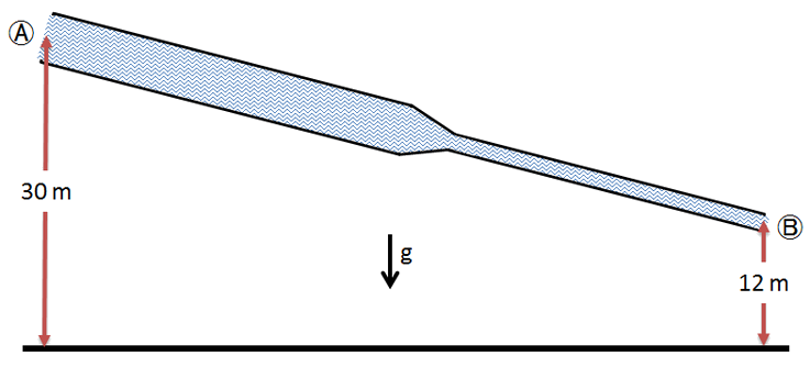
The fluid velocity at location Ⓐ is \(\SI{5}{m/s}\) and there are no frictional losses.

What is the fluid velocity at location Ⓑ ?

What is the relationship between the pipe diameters at locations Ⓐ and Ⓑ ?

Solution

The mechanical energy equation¶

Let’s now consider a more general case involving our conservation of energy equation. We will still consider steady-state conditions, but also assume that

mechanical effects (e.g., work) are not negligible, but do dominate thermal effects (\(\dot W >> \dot Q\))
changes in density are insignificant (incompressible flow)

We also separate our work term into shaft and frictional components and express them as work per mass terms: \(w_{s}\) and \(w_{f}\), respectively.

The value of \(w_{s}\) will be positive when work is done on the fluid (e.g., by a pump) and will be negative when the fluid does work on its environment (e.g., in a turbine).

On the other hand, \(w_{f}\), which represents the work (per mass) done by the fluid to overcome friction (or alternatively, the energy that was lost to friction), is always positive.

Utilizing these definitions and assumptions, we can derive a mechanical energy balance between an inlet and outlet point or two points along a flow stream.

Mechanical energy equation for steady-state, incompressible flow

\[\left(\frac{P}{\rho} + \frac {1}{2} \, \alpha \, v_{avg}^{2} + g \, z \right)_{\text{out}} - \left(\frac{P}{\rho} + \frac {1}{2} \, \alpha \, v_{avg}^{2} + g \, z \right)_{\text{in}} = w_{s} - w_{f}\]

or, considering an upstream point \(1\) and downstream point \(2\),

\[\left(\frac{P}{\rho} + \frac {1}{2} \, \alpha \, v_{avg}^{2} + g \, z \right)_{2} - \left(\frac{P}{\rho} + \frac {1}{2} \, \alpha \, v_{avg}^{2} + g \, z \right)_{1} = w_{s} - w_{f}\]

Unlike in the previous examples using the Bernoulli equation, we now consider cases where the frictional and shaft work are not negligible. Common cases will involve frictional losses in pipes and other devices in a process and work done on the fluid by devices such as pumps.

Friction¶

Flows in pipes and through many process devices involve frictional losses.

In this course, we will not explore the details of how to compute these losses. However, for pipes, they are related to factors such as the pipe diameter and roughness and the fluid velocity and properties (density, viscosity).

Example:

To give us some rough insights, let’s imagine a fixed mass flow of a constant density fluid through a pipe of constant diameter.

These facts tell us that the inlet (\(1\)) and outlet (\(2\)) velocities should be equal (\(v_{1}=v_{2}\)).

Let’s further assume that the pipe has no elevation changes (\(z_{1}=z_{2}\)) and there is no shaft work on the system (\(w_{s}=0\)).

Our general mechanical energy equation, letting \(v=v_{avg}\) and \(\alpha=1\), is

\[\left(\frac{P}{\rho} + \frac {1}{2} \, v^{2} + g \, z \right)_{2} - \left(\frac{P}{\rho} + \frac {1}{2} \, v^{2} + g \, z \right)_{1} = w_{s} - w_{f}\]

Considering our specific system, this general equation reduces to

\[P_{2} = P_{1} - \rho \, w_{f}\]

Because \(w_{s}>0\) and \(P_{2} < P_{1}\), it is clear that the frictional work has lead to a pressure loss/drop in our pipe.

What is the general approach to overcoming this pressure loss for common CBE systems?

Pumps.

Pumps¶

Pumps are mechanical devices that move liquids. There are also devices (fans, blowers, and compressors) that move gases, but we won’t talk about them here. Pumps move liquids by generating a high pressure at the pump outlet, which pushes the liquid into the outlet pipe. Let’s see how a pump affects the pressures in a pipe.

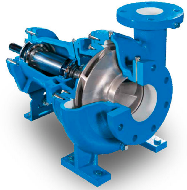
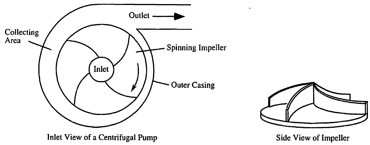
Types of pumps

Centrifugal pumps use the centrifugal force from a spinning disc-like impeller to produce liquid flow. The liquid enters the pump at 90° to the plane of the impeller and at the impeller center. The raised vanes on the impeller help to accelerate the liquid to the same speed as that of the impeller, which also forces the liquid to the collecting area around the periphery of the impeller and to the pump outlet.

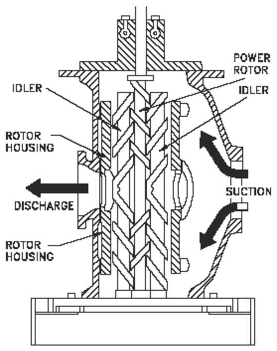
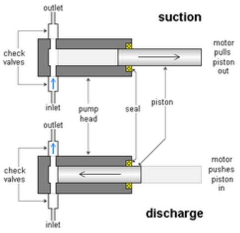
Positive-displacement pumps come in many varieties, but they all rely on mechanical parts to directly push the liquid. For example, one type of positive-displacement pump employs a piston that moves inside a cylinder, while inlet and outlet valves control the direction of liquid movement through the pump.

gear pump	screw pump	piston pump

Quantifying pump performance¶

First, we consider the amount of power required to overcome the various losses in the system. We will call this \(\text{Power}_{\text{delivered to the fluid}}\). This can be computed as follows:

Power required to be delivered to the fluid

\[\text{Power}_{\text{delivered to the fluid}} = \frac{\text{work}}{\text{time}} = \left(\frac{\text{mass}}{\text{time}}\right) \left(\frac{\text{work}}{\text{mass}}\right) = \dot m \, w_{s} = \rho \, \dot V \, w_{s}\]

The above is the power required by the system. However, a real pump cannot convert all of the input power directly to work on the fluid. Therefore, we must account for the pump efficiency:

\[\epsilon = \text{Efficiency} = \frac{\text{Power}_{\text{delivered to the fluid}}} {\text{Power}_{\text{to operate the pump}}}\]

The efficiency as defined by the above equation is always less than 1.0 (100%) for real systems. Typical values for the efficiency, \(\epsilon\), of a centrifugal pump range from 0.7 to 0.9 (70% to 90%).

Actual power required to operate a pump

\[\text{Power}_{\text{to operate the pump}} = \frac{\text{Power}_{\text{delivered to the fluid}}}{\epsilon} = \frac{\dot m \, w_{s}}{\epsilon}\]

When sizing a pump, there are two common power units: horsepower (hp), and kilowatts (kW). Here are a couple of useful conversion factors:

\[ \begin{align}\begin{aligned}\SI{1}{hp} = \SI{550}{ft.lb_{f}/s}\\\SI{1}{hp} = \SI{0.746}{kW}\end{aligned}\end{align} \]

Exercise: Sizing a pump for flow through an inclined pipe

Recall that our mechanical energy balance is

\[\left(\frac{P}{\rho} + \frac {1}{2} \, \alpha \, v_{avg}^{2} + g \, z \right)_{2} - \left(\frac{P}{\rho} + \frac {1}{2} \, \alpha \, v_{avg}^{2} + g \, z \right)_{1} = w_{s} - w_{f}\]

When applying this equation, it is important to remember that we must choose locations such that point \(1\) is upstream of point \(2\).

Consider the earlier example, but now we would like to move the flow against gravity from point Ⓑ to point Ⓐ, maintaining the mass flow rate through the pipe at \(\SI{7}{kg/s}\).

As in the earlier exercise, locations Ⓐ and Ⓑ are maintained at the same pressure.

The diameter of the pipe at location Ⓐ is \(\SI{12}{cm}\), while that at Ⓑ is \(\SI{4}{cm}\).

The frictional work per mass required is \(w_{f} = \SI{150}{m^{2}/s^{2}}\).

1. What is the fluid velocity at points Ⓐ and Ⓑ?

2. Assuming an efficiency of \(\epsilon = 0.8 \, (80 \text{%})\), what size pump (in units of \(\si{hp}\)) would be required?

You may assume that the velocity adjustment factor is unity (\(\alpha=1\)).