|
|
HYDROLOGICAL AND SEDIMENT PROCESSES | ||||||||||||||||||||||||||||||||||||
|
Flow Routing | |||||||||||||||||||||||||||||||||||||
|
|
The rainfall intensity might be assumed to be uniform. In this case, the rainfall intensity and duration are needed as input to the program. When more than one rain gage is used in the estimation of the precipitation, an interpolation scheme based on the inverse distance squared approximates the distribution of rainfall intensity over the watershed:
where, it(j,k) = rainfall intensity in element (j,k) at time t imt(jrg,krg) = rainfall intensity recorded by the m-th rainfall gage located at (jrg,krg) dm = distance from element (j,k) to m-th rain gage located at (jrg,krg) NRG = total number of rain gages
As rain falls on a vegetated surface, part of it is held on the foliage by surface tension forces. Rather than reaching eventually the ground, this portion of the rainfall evaporates directly and does not take part in ultimate runoff and thus, it is usually termed interception loss (Eagleson 1970). Chow et al. (1988) defined retention the part of the surface storage held for a long period of time and depleted by evaporation. Because intercepted water does not reach the soil surface, it has no part in infiltration. Accordingly, the interception depth is subtracted from the rainfall before infiltration is calculated. In CASC2D, the rainfall rate is reduced until the interception depth (I) has been satisfied. For a given grid cell inside the basin, if the total rain falling during the first time increment (dt) is greater than I, the rainfall rate is reduced by I/dt. If the rainfall depth is less than I, the rainfall rate is set to zero and the remainder of the interception is removed from the rainfall in the following time increments. Measured values of interception depth for a number of vegetative covers are found in Woolhiser et al. (1990) and Bras (1990).
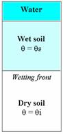
The Green & Ampt (1911) equation provides the primary relationship for infiltration within the CASC2D computer model. The Green and Ampt infiltration scheme gained considerable attention partially due to the ever growing trend of physically-based hydrological modeling (Philip 1983). To accurately account for the physical process involved with surface flow, CASC2D uses the Green and Ampt approximation for soil infiltration. Specifically, this relationship is utilized within the model’s infiltration scheme to determine the depth and rate of soil infiltration as a component of the resulting overland flow. The Green-Ampt model assumes piston flow with a sharp wetting front between the infiltration zone and soil at the initial water content. The wet zone increases in length as infiltration progresses (Bras 1990). Neglecting the level of ponding on the surface, the general equation showing the Green-Ampt relationship can be expressed as (Bras 1990).
where: f = infiltration rate Ks = saturated hydraulic conductivity Hf = capillary pressure head at the wetting front Md = soil moisture deficit = (qe - qi) qe = effective porosity = (j - qr) j = total soil porosity qr = residual saturation qi = soil initial moisture content F = total infiltrated depth To apply this calculation to the entire watershed area, four separate physical characteristics must be known and provided as input to the model. These characteristics are hydraulic conductivity, capillary pressure, effective soil porosity, and initial soil moisture content. Their numerical values can be obtained from the experimental data by Rawls et al. (1983) depending on the soil texture.
The governing equations for overland flow with the CASC2D Model are based primarily on the de-Saint Venant Equations of continuity and momentum. Using these formulations, CASC2D was designed around an explicit finite difference, diffusive-wave method to route overland flow. The general form for these equations, as shown in Julien and Saghafian (1991), are commonly expressed in partial differential form as: Continuity:
Momentum: x-direction
y-direction
where: h = surface flow depth qx = unit flow rate in the x-direction, qy = unit flow rate in the y-direction e = excess rainfall (i-f) i = rainfall intensity f = infiltration rate x,y = Cartesian spatial coordinates t = time So(x,y) = bed slopes in the x- and y-direction, respectively Sf(x,y) = friction slopes in the x- and y-direction, respectively u,v = average velocities in the respective x- and y- directions g = gravitational acceleration Equations 4 and 5 show the relationship between the net forces per unit mass in each direction and the acceleration of flow in relation to that given direction. Thus, the forces along a given axis are shown on the right side of the equation, while the local and convective acceleration is given by the left-hand side of the equation. The simplified diffusive approximation for Equations 4 and 5 assumes that the net forces acting along the given axis of interest are approximately zero. Thus, the resulting diffusive wave approximation can be descried by the following equations.
The key advantage that is provided in using the diffusive form of the momentum equations is the ability to account for backwater effects observed during overland and channel flow events. Using the three equations given for continuity and momentum, a resistance law can be established. This equation relates flow rate to depth and other given flow parameters such as surface roughness. The defined resistance law can be derived for either the x or y-directions as:
In this form ax,y and b are flow regime parameters that vary depending on whether turbulent or laminar conditions exist. CASC2D assumes turbulent conditions for the entire watershed and the Manning approximation for ax,y and b are determined to be:
Where n is the Manning roughness coefficient, or surface roughness. This coefficient can be estimated from the land use map using the values provided by Woolhiser (1975). The initial and boundary conditions applied for a plane of length L are respectively:
The channel routing scheme employed by CASC2D is capable of processing completely unsteady hydraulic scenarios. This is achieved by the use of a one-dimensional diffusive channel flow equation (Julien and Saghafian 1991). The governing equations for the channel flow routing process are similar to those for overland flow, with one significant exception to note. The equations used in channel flow routing are defined by a finite width established for a given channel section. The one-dimensional continuity relationship can be expressed by the following equation (Julien and Saghafian 1991):
where: A = channel flow cross-sectional Area Q = total channel discharge ql = lateral inflow rate per unit length (into or out of the channel) Once again, by assuming the flow within the channel is completely turbulent, the model utilizes Manning’s equation to ascertain a value for channel flow equation (Julien and Saghafian 1991).
where: R = hydraulic radius Sf = friction slope n = Manning roughness coefficient
Base flow is the component of streamflow that can be attributed to ground-water discharge into streams. In CASC2D-SED the base flow is accounted for by defining an initial water depth in channel cells of the input base depth grid. If an initial water depth is defined in overland cells, this may represent lakes or the ponding of water from previous rainfall events. Home | Registration | Background | Processes | References | Example | Download | Feedback Department of Civil and Environmental Engineering - Colorado
State University |