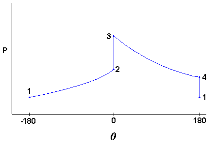
The cycle is named after a German, Nikolaus Otto, who built the first spark ignition engine in 1876. Figure 4 shows schematically how the pressure varies during compression and expansion. From -180 degrees (bottom dead center) to 0 degrees (top dead center) the upward motion of the piston compresses the air/fuel mixture. The heat input for this model is assumed to occur entirely at top dead center. From 0 degrees to +180 degrees the expanding gases move the piston downward and produce work. The heat rejection for this cycle model is assumed to occur entirely at bottom dead center.

The air standard Otto cycle is modeled as a closed system with a fixed air/fuel mass, and uses the following process assumptions:

1-2 Compression which is reversible and adiabatic
2-3 Heat addition from fuel
3-4 Expansion which is reversible and adiabatic
4-1 Heat rejection to cylinder walls

First Law Analysis of the Otto Cycle

Using the first law:
 

Process 1-2:

Since the process is reversible and adiabatic it is also isentropic, which leads to:

Process 2-3:

Process 3-4:

Process 4-1:

In an ideal engine all the fuel is consumed in combustion.  Realistically this is not the case there will alwalys be some amount of fuel that will be left unburned. Due to this residual fuel remaining in the cylinder the intial and exhaust temperatures of the cycle will not retrun to thier inital value. Assuming the above definitions for the pressure and the temperature at given points in the cycle, the residual mass fraction can be given by:

    Where:
            T_e    =    exhaust temperature
            P_e    =    exhaust pressure
            r       =    compression ratio

In order to determine the residual mass fraction, the exhaust pressure and temperature must be known.  The exhaust pressure is typically half of the intake pressure, P_i = 2P_e.  The exhaust temperature can be determined by assuming that the final mass in the cylinder expands isentropically to the exhaust pressure.

Using the relationships developed for temperatures and pressures from the first law analysis, the exhaust temperature and residual mass fraction can be determined by iterating.  The Residual Mass Fraction Applet performs this iteration in order to determine T_e and f, given inital guess for Te and f.

Thermal Efficiency Derivation

The overall efficiency for the cycle (indicated thermal ) is given by:

since

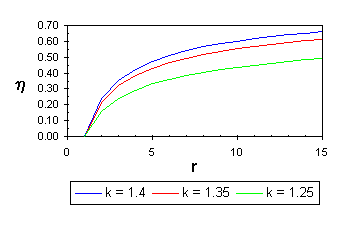
The following relationship for the efficiency can be developed and plotted against the compression ratio in Figure 5.

A typical value for an air/fuel mixture is k = 1.35.