This article describes some observations about the data on a newer Dodge Ram pickup. The data are from a simple vehicle dynamics tests from a drive around the block. The work here assumes no prior knowledge of the meaning or interpretation of CAN messages. The following signals are desired in this work:
Some of these signals need more study to determine attribution (i.e. we do not know which of the wheel speeds correspond to each wheel). Also, only the raw data are presented, so calibration is needed to analyze CAN data using engineering units.
Dodge is nice enough to publish the electrical wiring diagrams for their work vehicles from 2004 and newer online at http://www.dodge.com/bodybuilder/year.pdf. Select the year, select the vehicle, and select the body style. The year of interest may be incomplete if there were no major redesigns for that model year. For example, to get the wiring diagram for a 2010 Ram, you may need to examine the diagrams for the 2009.
Also, check out http://www.rambodybuilder.com/ for newer information.
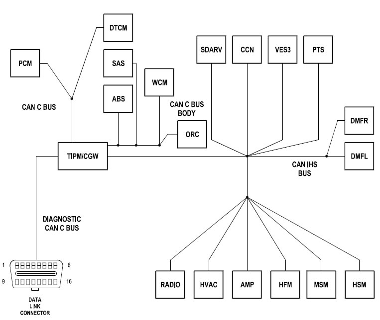
In the Bus Communications diagram, the overall picture is shown below with three distinct CAN bus circuits: Diagnostic CAN, the high-speed CAN C, and the low-speed CAN IHS or "Comfort CAN".
The high speed CAN runs at 500kbps and the comfort CAN runs at 125kpbs. Both use 11-bit identifiers.
The first attempt to access the CAN bus was through the diagnostic port. However, no live data was present. Clearly from the picture above, the CAN C network contains the live data that is shared among the electronic control modules. The following diagram shows part of the CAN C network.
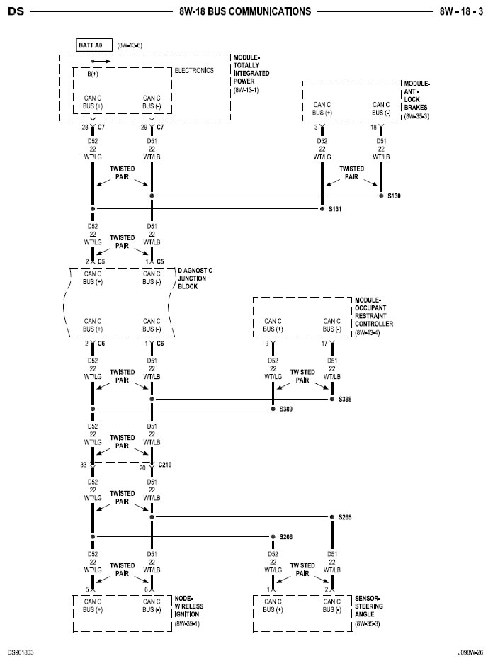
This diagram shows the CAN C bus is made from two twisted pair wires that are 22 gauge in diameter. The CAN C Bus (+) wire is white with a light green stripe and the CAN C Bus (-) is white with a light blue stripe. Interestingly, the diagnostic port uses a twisted pair of white with dark stripes. So if two sets of white striped twisted pairs are in the same bundle, the twisted pair with the lighter stripes will be the CAN C bus that has the live data. In summary:
CAN C (+): white with a light green stripe
CAN C (-): white with a light blue stripe
The following photo is taken of the wires that are available near the driver's side firewall in the engine compartment. The red material is liquid electrical tape that was applied after the CAN communication wires have been tapped.
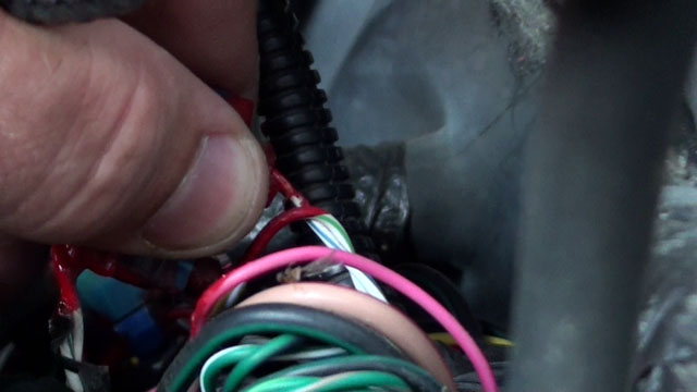
With physical access to the network, the network traffic can be monitored and recorded.
With the network monitored, external measurements are needed to correlate signals. For this a Racelogic VBox 3i was used to record the vehicle speed. The following speed record was obtained.
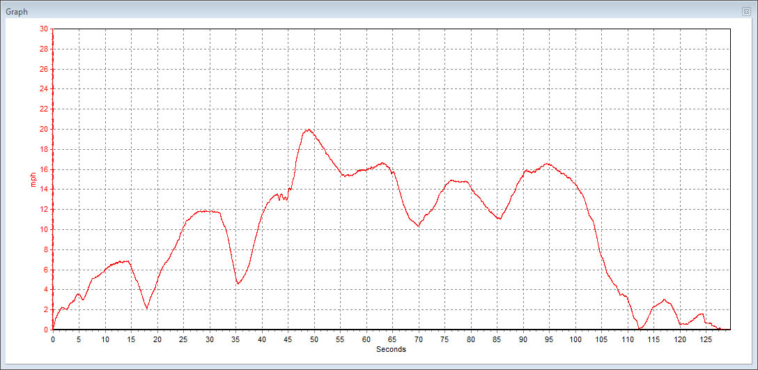
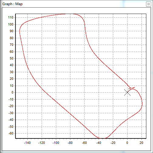
The test sequence started with a pickup poised to drive away from a normal residential driveway. After pulling out of the driveway, a series of right hand turns were made to complete the route. Then the pickup was backed into the parking space. The map of the path of travel with the X marking the starting position on the time graph is shown below.
The CAN data from the 500k CAN bus was captured using a Dearborn Group Gryphon S3, which is out of production and replaced by the Beacon product. The 14Mb raw data file is in a comma separated value format as exported by the DG Technologies Hercules software. Since this data file is large and contains all message traffic, decoding it seems like a daunting task. However, the messages are broadcast using an ID and the ID usually determines what purpose the message has. Therefore, if we can filter by ID, then we can examine the data more efficiently. By efficiently, we mean using plotting tools to generate patterns that can match the dynamic signals measured with external devices. To this end, we created a Python program that takes advantage of the matplotlib tools that parses the CAN data, filters by ID, and plots many combinations of the data. The Python program to decode the data record is described in the next section.
Since it is difficult to evaluate data in a time series by looking at hexadecimal numbers, a method to visualize the data was needed. To this end, a python program was written to parse a CAN data file from the Gryphon S3. The first section of the program evaluates all the CAN IDs, data lengths, and their nominal frequency. For this example, the script produced three pdf files with graphic representations of various byte combinations.
Byte Plots For Drive Around The Block.pdf
Even Byte Plots For Drive Around The Block.pdf
Odd Byte Plots For Drive Around The Block.pdf
There are 55 unique IDs in the log file that are summarized in the following table. The timing data in the table below is approximate. Byte counts start at 0 and go to 7 for an 8 byte message.
| CAN ID (Hex) | CAN ID (Dec) | Data Length | Frequency (Hz) | Period (sec.) | Notes |
|---|---|---|---|---|---|
| 0A0 | 160 | 1 | 10.0173 | 0.0998271 | |
| 101 | 257 | 4 | 7.49224 | 0.133472 | |
| 111 | 273 | 6 | 0.00488412 | 204.745 | |
| 1C0 | 448 | 6 | 5.02087 | 0.199169 | |
| 1C6 | 454 | 7 | 0.99636 | 1.00365 | |
| 1D0 | 464 | 6 | 0.781459 | 1.27966 | |
| 1E6 | 486 | 7 | 0.99636 | 1.00365 | |
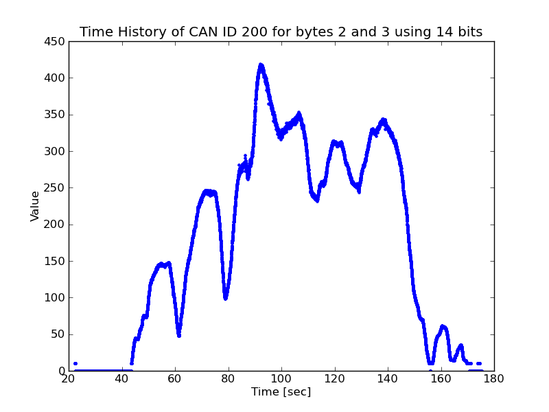
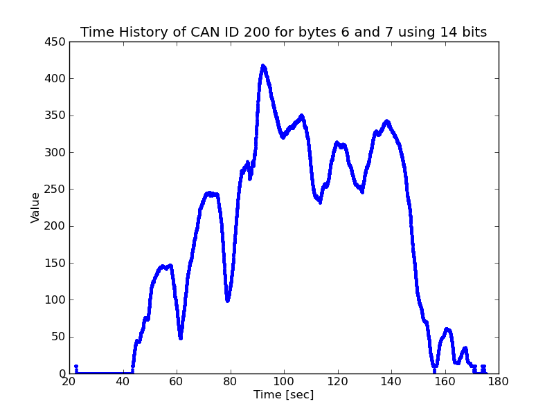
| 200 | 512 | 8 | 37.3586 | 0.0267676 | Speed like signals on Bytes 2-3, 4-5 and 6-7 |
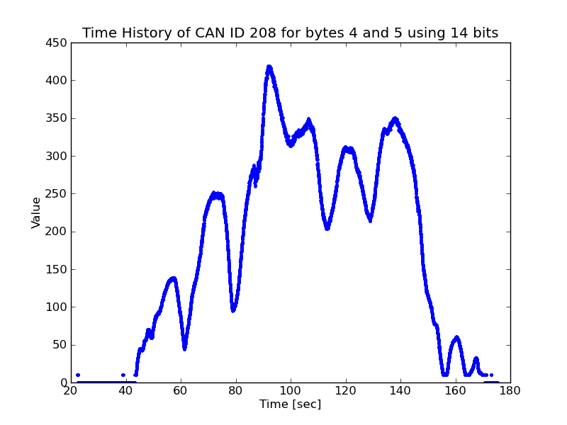
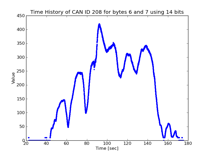
| 208 | 520 | 8 | 37.3586 | 0.0267676 | Speed like signals on Bytes 4-5 and 6-7 |
| 210 | 528 | 8 | 37.4514 | 0.0267013 | Byte 2 has brake pressure like signals |
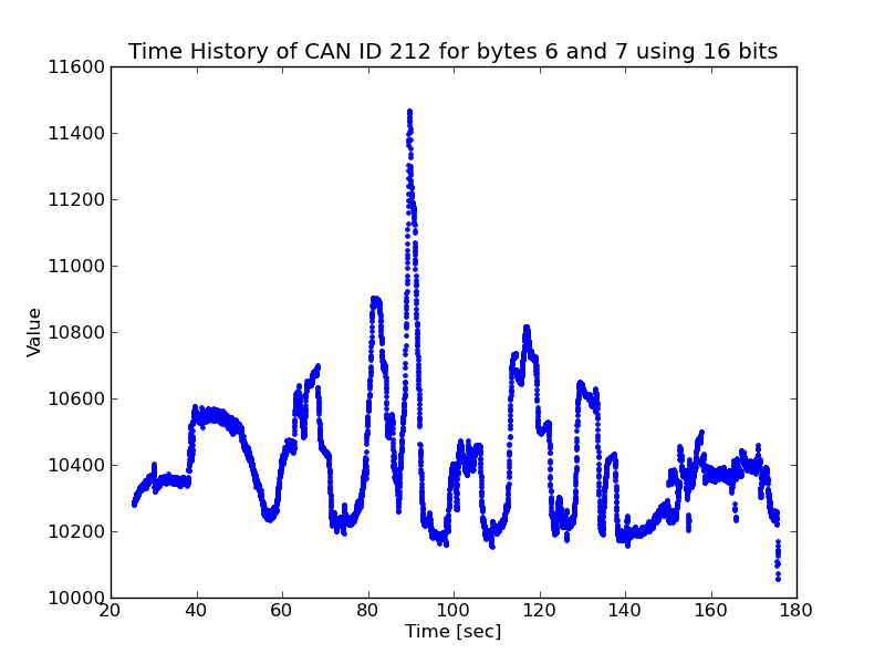
| 212 | 530 | 8 | 37.4514 | 0.0267013 | |
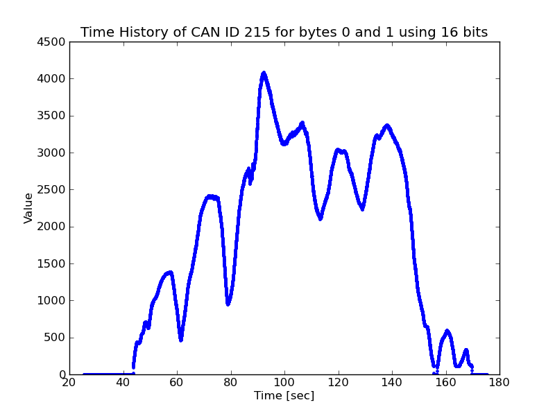
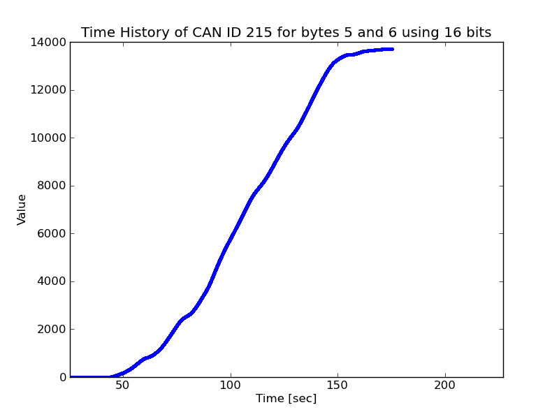
| 215 | 533 | 7 | 37.3635 | 0.0267641 | Speed like signal on bytes 0-1 |
| 218 | 536 | 8 | 37.4514 | 0.0267013 | |
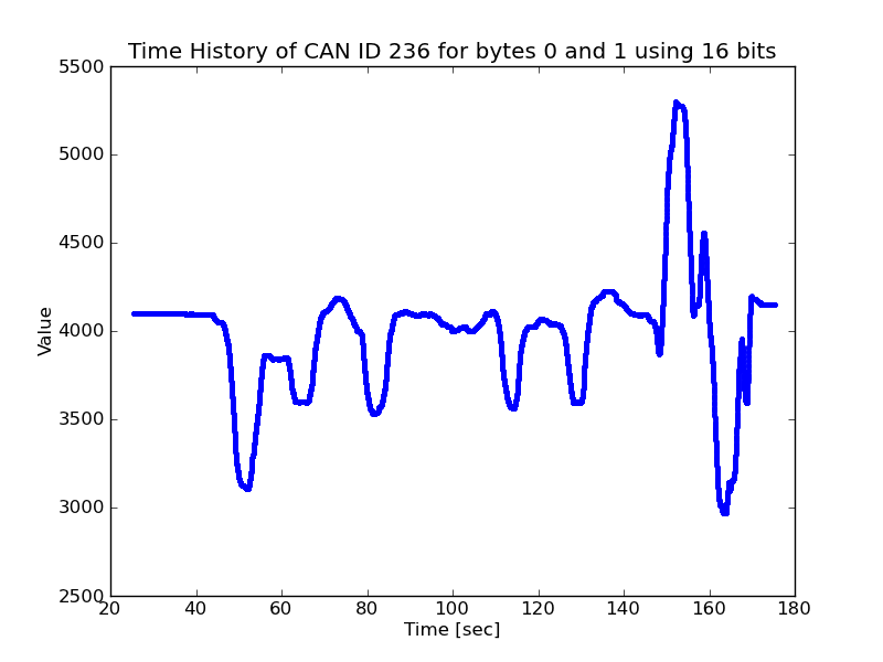
| 236 | 566 | 8 | 74.6781 | 0.0133908 | Steering data on 0-1 |
| 248 | 584 | 8 | 49.9889 | 0.0200044 | |
| 300 | 768 | 8 | 37.3635 | 0.0267641 | Signed signal for 6-7 |
| 308 | 776 | 8 | 74.9028 | 0.0133506 | |
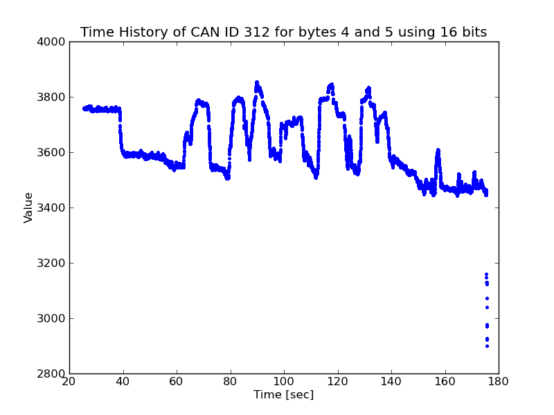
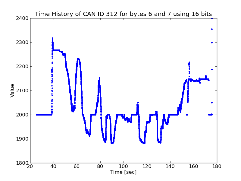
| 312 | 786 | 8 | 74.9028 | 0.0133506 | Engine like data |
| 315 | 789 | 6 | 49.9889 | 0.0200044 | |
| 325 | 805 | 7 | 49.9889 | 0.0200044 | |
| 328 | 808 | 8 | 37.3635 | 0.0267641 | Byte 2 |
| 330 | 816 | 8 | 37.3635 | 0.0267641 | |
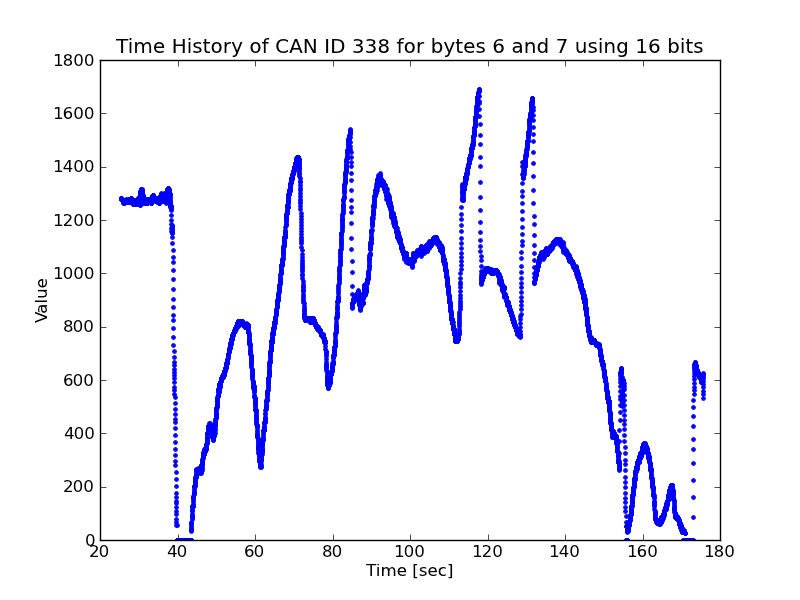
| 338 | 824 | 8 | 37.4514 | 0.0267013 | Speed on 0-1, 6 and 7 (maybe steering?) |
| 358 | 856 | 8 | 37.3488 | 0.0267746 | |
| 392 | 914 | 8 | 9.99779 | 0.100022 | |
| 3D0 | 976 | 4 | 7.49224 | 0.133472 | Bytes 0 and 1 have different dynamic data |
| 3E4 | 996 | 3 | 0.99636 | 1.00365 | Bytes 1 and 2 are distance like signals |
| 3E6 | 998 | 1 | 1.9976 | 0.5006 | |
| 3FB | 1019 | 5 | 1.00613 | 0.993909 | |
| 3FD | 1021 | 8 | 0.49818 | 2.00731 | |
| 3FF | 1023 | 6 | 19.9956 | 0.0500111 | Dynamic on Byte 0 |
| 408 | 1032 | 8 | 9.99779 | 0.100022 | |
| 410 | 1040 | 8 | 49.9889 | 0.0200044 | Low resolution dynamic on byte 1 |
| 415 | 1045 | 7 | 7.49224 | 0.133472 | Dynamic signal on byte 1 |
| 418 | 1048 | 8 | 37.4514 | 0.0267013 | |
| 428 | 1064 | 7 | 37.3488 | 0.0267746 | |
| 445 | 1093 | 6 | 16.6646 | 0.0600074 | Dynamic level sensor like data on 0 |
| 4A0 | 1184 | 8 | 7.49224 | 0.133472 | All dynamic signals |
| 4D0 | 1232 | 4 | 0.99636 | 1.00365 | |
| 520 | 1312 | 4 | 7.49224 | 0.133472 | |
| 5B0 | 1456 | 8 | 2.00737 | 0.498164 | |
| 5FE | 1534 | 8 | 0.99636 | 1.00365 | |
| 608 | 1544 | 8 | 7.48735 | 0.133559 | Dynamic signals on bytes 0, 5, and 6 |
| 67F | 1663 | 8 | 0.49818 | 2.00731 | |
| 6F9 | 1785 | 6 | 0.49818 | 2.00731 | |
| 6FA | 1786 | 8 | 7.48735 | 0.133559 | |
| 6FD | 1789 | 8 | 0.49818 | 2.00731 | |
| 6FE | 1790 | 8 | 7.48735 | 0.133559 | |
| 6FF | 1791 | 8 | 1.9976 | 0.5006 | |
| 700 | 1792 | 8 | 3.57029 | 0.280089 | |
| 702 | 1794 | 8 | 3.57517 | 0.279707 | |
| 706 | 1798 | 8 | 3.57029 | 0.280089 |
The following figures contain dynamic signals extracted from the CAN data. These are contained within the pdf documents generated by the Python script. There were 6 different speed signals that match the pattern from the VBox record.

The following is likely an accelerator pedal signal.
Steering like signals:
RPM like signals:
Distance signals:
The following signals are unknown:
In summary, there are many signals on the CAN that contain dynamic signals that can be useful for studying vehicle dynamics. The data presented so far has not been calibrated. However, identifying messages of interest is the first step.