ECE411
Homework #3
Reading: Chapters 5 and 6 and Sections 7.1-7.6 of Chapter 7
Questions:
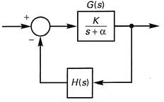
1. Consider the system below. The parameter a has a nominal value of 10.
(a)
With H = 0 (open-loop system), find the sensitivity of closed-loop transfer
function T(s) to a; that is find SaT about the nominal value of a.
(b)
Repeat (a) for H(s) = 1.
(c) Sketch the magnitude of the sensitivity
functions of (a) and (b) as a function of frequency for K=1. Indicate the system’s bandwidth.
(d)
Repeat (c) for K=100, and note the effects of sensitivity of (i) closed-loop
versus open-loop; (ii) high loop-gain versus low loop-gain for the closed-loop
system.
2. Consider the system below. It is assumed that the sensor modeled as the
gain Hk is perfect; that is, the signal out of Hk is the
perfect measurement of c(t). The
inaccuracies of the physical sensor are represented by the disturbance d(t),
and the sum of the perfect measurement and d(t) is the output of the physical
sensor. This is a commonly used model
for sensor inaccuracies.
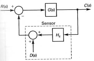
(a)
Express C(s) as a function of both the system input and the disturbance input.
(b)
Assume that the input r(t) is a constant.
What is the property required of G(s) such that the steady-state gain
from r(t) to c(t) is unity? Let Hk
= 1.
(c)
Assume that G(s) has the property found in (b), and Hk = 1. Assume that the sensor inaccuracy d(t) is
modeled as a constant signal. Find the
steady-state gain from d(t) to c(t). We see from this problem why the sensor
should be made as accurate as possible.
3. Shown below is the control system for one
joint of a robot arm. The controller is
a PD compensator. This robotic control
system is described in Chapter 2 of the text.
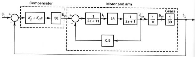
(a)
Calculate the plant transfer function from Ea(s) to Q(s).
(b)
Find the ranges of the compensator gains Kp and KD, with
these gains positive, such that the closed-loop system is stable.
(c)
Let KD = 1. Find Kp
such that the system will have a steady-state oscillation, and find the period
of that oscillation.
4. Consider the system below. Note that the sensor gain is not unity.
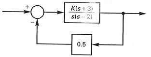
(a)
Accurately sketch the root locus of the system.
(b)
Find any points at which the locus crosses the jw axis. Use the Routh-Hurwitz criterion as required.
(c)
From (a) and (b) find the range of K for which the system is stable.
(d)
From (a) and (b) find the range of K for which the system is stable and the
closed-loop transfer function poles are real.
(e)
From the results above, find all the values of gain for which the system is
critically damped.
5. Sketch the root locus of the single-loop
systems having the open loop functions KG(s)H(s) given by the following
functions. Solve for the values of s at
any crossings of the imaginary axis.
(a)
K(s+1)/s2
(b)
K/[s(s+2)2]
(c)
K/{s[(s+10)2 + 1]}
(d)
K/{s[(s+5)2 + 25]}
(e)
Verify each root locus with MATLAB and all jw-axis crossings with
SIMULINK.
6. Consider the PD compensator below, which adds
a zero to the system open-loop function.

(a)
To show the effects of the compensator, sketch the root locus given a zero in
the following ranges:
(i) –a > 0
(ii) -2 < -a < 0
(iii) –a < -2
(b)
Which of the three cases above will result in the system with the fastest
settling time?
(c)
Which of the three cases above can result in an unstable system?