ECE411 Lab Exercise #2

Introduction to Simulink

Objectives

This laboratory exercise is intended to provide a tutorial introduction to Simulink. Simulink is a Matlab toolbox for analysis/simulation of interconnections of dynamic systems, and it will be used heavily throughout the rest of the course/lab. All the exercises in this assignment can be done entirely in Matlab/Simulink.

1) Running, Plotting, Printing: In order to see a demonstration Simulink diagram, type sldemo_househeat at the Matlab prompt. Open the scope block, labeled “PlotResults” by double clicking, and then run the simulation using the buttons or pull down menus provided.

Print the plot of the simulation output (scope block) and print the simulation model itself.

2) Model Building: Figure 1 shows a Simulink model which represents the motor gear system in the Controls lab, with a PID controller implemented in feedback around it. Launch the simulink library browser from within Matlab by using the button or typing simulink. Then open a new model (using button or pull down menus), and build a coy of the above model. This is achieved by dragging components from the library to the model and connecting them using the mouse. Double clicking a box then allows you to edit the components, such as entering values for the Transfer function (as shown). For the PID block, set the proportional gain to 0.05, and the integral and derivative gains to zero.

Look around at the many available blocks in Simulink. You will certainly need to look in Sources, Sinks, Continuous, Math, Signals & Systems, as well as Additional Linear under Simulink Extras for the PID controller.

Note that there is no block for “Pulse Input”, but that has been made for you from basic components using the Create Subsystem command under Edit. The contents of the box are shown in figure 2. You can even use the Mask Subsystem command to generate your own library blocks.

When you have built a copy of the model, save it with the name “gear”. (It will actually be saved as gear.mdl.) You can then launch this model later from Matlab simply by typing gear at the command line. Go under Simulation to Parameters and set the simulation time to 8 seconds.

Run the simulation and print the results from the scope block. You should get a plot like figure 3, which shows the commanded response and actual system response (note the autoscale button on the scope). Note that in order to get the correct commanded responses you will need to enter the appropriate values for the two step input blocks that make up your pulse input.

Having completed this exercise, you should have a model plot and a simulation run that essentially reproduce the figures shown here. Now try varying the parameters of the PID controller and see how they affect the closed-loop control system (note that you can enter variable names in Simulink Blocks if you like, and it will read them from the Matlab workspace). You do not need to generate large numbers of plots, but Plot a few of the results and discuss how the different controller parameters (Proportional, Integral, and Derivative) affect the closed loop performance. See if you can manually tune the controller to get a good step response. Later in the semester we will revisit this problem with design tools we have learned in class, and try them out both in simulation (as here) and on the actual hardware.

Figure 1: Simulink model of motor gear drive system

Figure 2: Pulse input subsystem

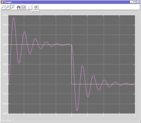
Figure 3: Gear Plot